Deep learning ensemble for brain tissue segmentation
A 2D and 3D CNN Ensemble Approach for MRI Segmentation
Authors: Frederik Hartmann, Xavier Beltran Urbano
Code: Github
Report: Github
*This project was carried out within the scope of the Medical Image Segmentation course taught by Prof. Dr. Xavier Lladó.
December 2023
Dataset
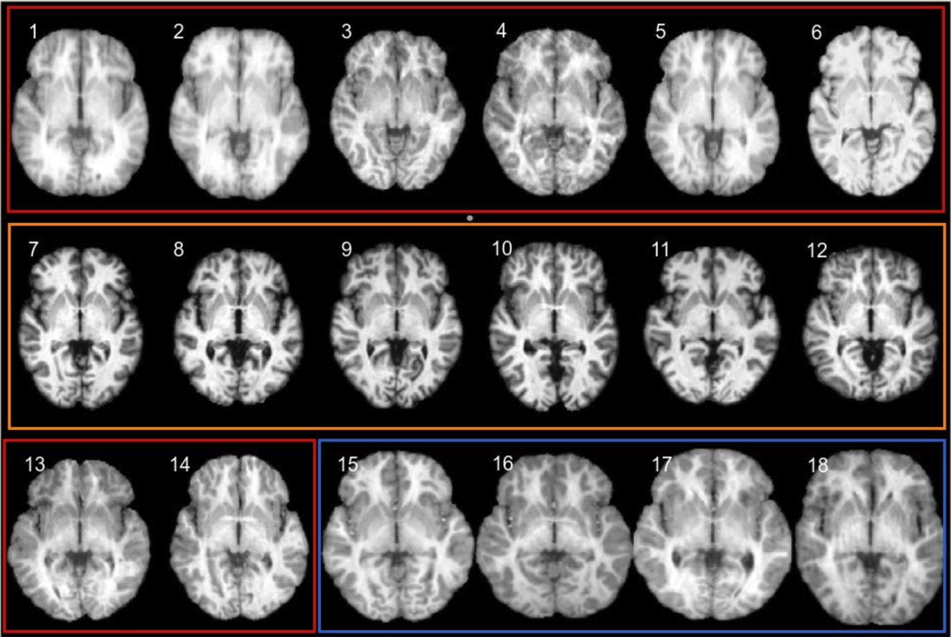
The dataset used in this study is the IBSR18, containing 18 T1-weighted scans of normal subjects from the Internet Brain Segmentation Repository (IBSR). It includes preprocessed scans with a 1.5 mm slice thickness and ground truth segmentation for white matter (WM), gray matter (GM), and cerebrospinal fluid (CSF).

Methodology
Our approach can be divided into 2 sections:
· Preprocessing
First, normalization was implemented using a robust z-normalization technique, chosen due to the non-Gaussian distribution and the presence of outliers in some data. This involves adjusting the intensity values by subtracting the mean (calculated using the 25th and 75th quantiles) and dividing by the standard deviation, calculated over the same quantile range. Additionally, data augmentation was performed through random flips and rotations of the original images to enhance algorithm reliability. Finally, selective slice selection was employed for multi-class segmentation, prioritizing slices containing cerebrospinal fluid (CSF) to address class imbalance.
· Training
For the training of this approach, several architectures, such as U-Net, Res-U-Net, Dense-U-Net, and SegResNet, have been used. We have also investigated the effect of utilizing distinct image planes (axial and coronal). Additionally, both 2D and 3D approaches have been analyzed. In Table 1, you can observe all the networks that we have trained independently. After the single trainings, we have ensembled the networks in different configurations (see Table 2).
Results
Both quantitative and qualitative results are presented in this section. They are as follows:
· Quantitative Results
In the following tables, we can observe the results obtained for the single trainings and the different ensemble methods carried out in this project. The metrics utilized to evaluate the segmentations are the Dice Coefficient (DSC) and the Hausdorff Distance (HD).
Single Model Results
| Model | CSF Dice | GM Dice | WM Dice | Mean Dice | CSF HD | GM HD | WM HD | Mean HD |
|---|---|---|---|---|---|---|---|---|
| 2D Coronal U-Net | 0.878 | 0.937 | 0.933 | 0.917 | 39.352 | 11.344 | 10.443 | 20.380 |
| 2D Coronal Dense U-Net | 0.899 | 0.937 | 0.938 | 0.925 | 17.168 | 12.199 | 8.149 | 12.502 |
| 2D Coronal Multi-U-Net | 0.890 | 0.935 | 0.936 | 0.920 | 26.234 | 13.391 | 8.422 | 16.016 |
| 2D Coronal Res-U-Net | 0.882 | 0.931 | 0.931 | 0.915 | 21.894 | 12.000 | 10.905 | 14.933 |
| 2D Axial U-Net | 0.868 | 0.929 | 0.922 | 0.906 | 26.598 | 9.876 | 9.887 | 15.454 |
| 2D Axial Dense-U-Net | 0.868 | 0.920 | 0.920 | 0.902 | 27.137 | 11.281 | 10.580 | 16.333 |
| 2D Axial Multi-U-Net | 0.876 | 0.923 | 0.926 | 0.908 | 30.938 | 10.546 | 9.872 | 17.119 |
| 2D Axial Res-U-Net | 0.866 | 0.925 | 0.921 | 0.904 | 23.733 | 21.277 | 10.113 | 18.375 |
| 2D Seg-Res-Net | 0.877 | 0.933 | 0.935 | 0.915 | 13.540 | 9.977 | 9.449 | 10.989 |
| 3D U-Net | 0.882 | 0.942 | 0.942 | 0.922 | 16.202 | 12.864 | 11.574 | 13.486 |
| 3D Seg-Res-Net | 0.888 | 0.935 | 0.937 | 0.921 | 15.198 | 10.367 | 9.541 | 11.702 |
| SynthSeg | 0.812 | 0.829 | 0.888 | 0.843 | 29.822 | 8.353 | 12.066 | 16.747 |
Ensemble Results
| Model | CSF Dice | GM Dice | WM Dice | Mean Dice | CSF HD | GM HD | WM HD | Mean HD |
|---|---|---|---|---|---|---|---|---|
| The Coronal Ensemble Mean | 0.895 | 0.939 | 0.939 | 0.925 | 18.508 | 9.630 | 7.783 | 11.974 |
| The Coronal Ensemble Maximum | 0.893 | 0.939 | 0.939 | 0.923 | 23.860 | 9.811 | 8.843 | 14.171 |
| The Coronal Ensemble Majority | 0.890 | 0.939 | 0.937 | 0.922 | 19.123 | 11.465 | 7.564 | 12.717 |
| The Axial Ensemble Mean | 0.884 | 0.930 | 0.928 | 0.914 | 17.121 | 10.704 | 9.127 | 12.317 |
| The Axial Ensemble Maximum | 0.881 | 0.930 | 0.927 | 0.913 | 23.055 | 10.655 | 9.782 | 14.498 |
| The Axial Ensemble Majority | 0.877 | 0.930 | 0.925 | 0.911 | 22.114 | 10.946 | 9.277 | 14.112 |
| The Coronal + Axial Mean | 0.897 | 0.939 | 0.938 | 0.925 | 16.410 | 8.902 | 9.095 | 11.469 |
| The Coronal + Axial Maximum | 0.893 | 0.938 | 0.937 | 0.923 | 21.901 | 10.270 | 9.370 | 13.847 |
| The Coronal + Axial Majority | 0.894 | 0.940 | 0.938 | 0.924 | 16.611 | 9.811 | 8.653 | 11.692 |
| The Multidimensional Ensemble Mean | 0.904 | 0.945 | 0.948 | 0.932 | 11.918 | 8.730 | 7.660 | 9.436 |
· Qualitative Results
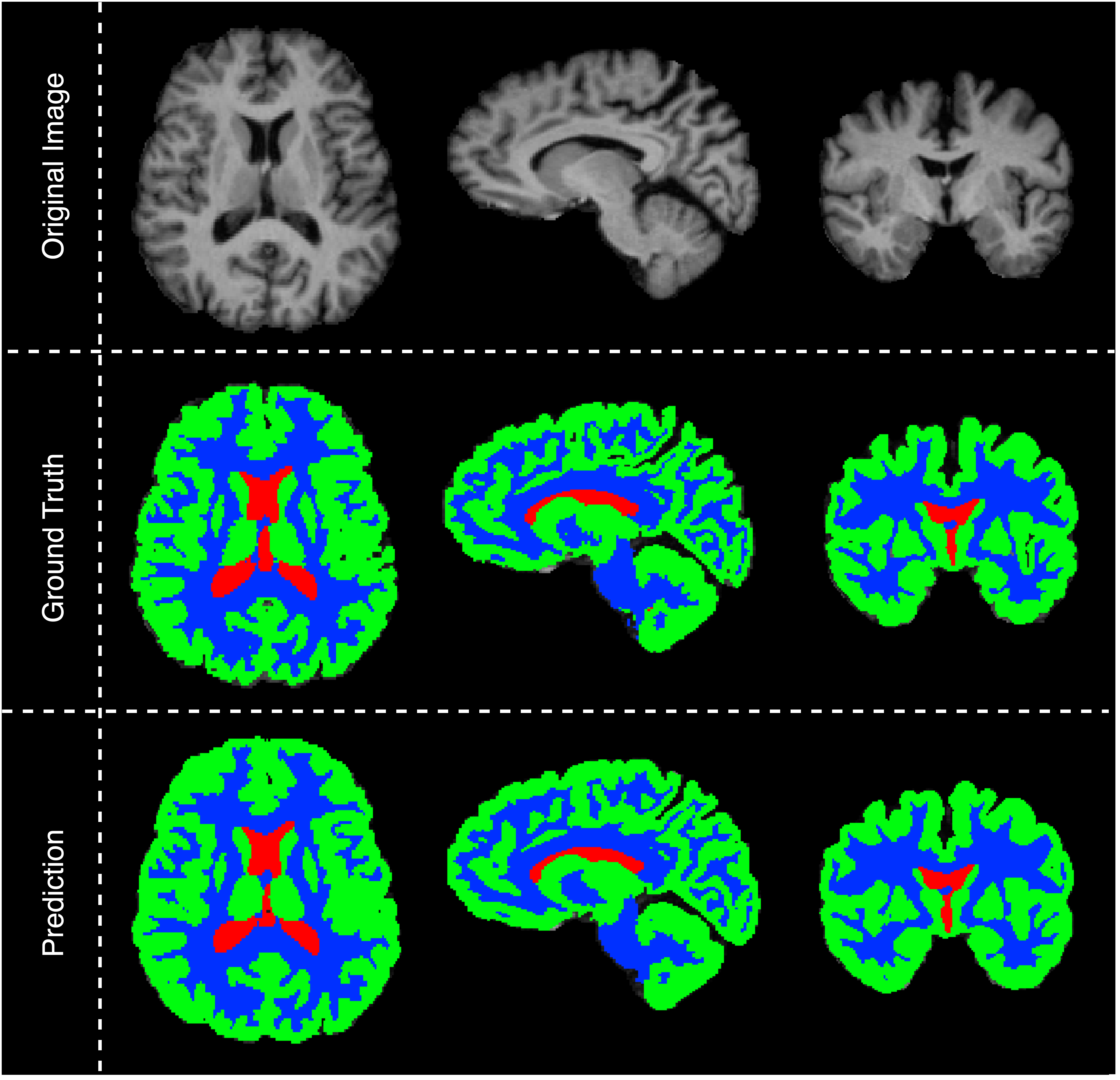
Here, an example of the segmentation obtained from the ensemble with the best performance (the Multidimensional Ensemble Mean) is presented in Fig 2.

Conclusion
The study clearly illustrates the efficacy of an ensemble methodology that synergizes 2D and 3D convolutional neural networks (CNNs) for segmenting brain tissue. This innovative approach benefits significantly from leveraging various orientations of 2D slices in combination with both 2D and 3D models. Among the various techniques explored, the ensemble method, especially the mean of probabilities technique, stands out for its exceptional robustness and precision in results. Future scope would include working on dealing with the imbalance problem since, even after obtaining excellent performance for all tissues, it can be appreciated that the results obtained for CSF are slightly lower than the WM and GM ones.