A new brain atlas
A brain atlas from scratch
Authors: Frederik Hartmann, Xavier Beltran Urbano
Code: Github
Report: Github
This project was carried out within the scope of the Medical Image Registration course taught by Prof. Dr. Robert Martí. You can reach a detailed report here.
November 2023
Dataset
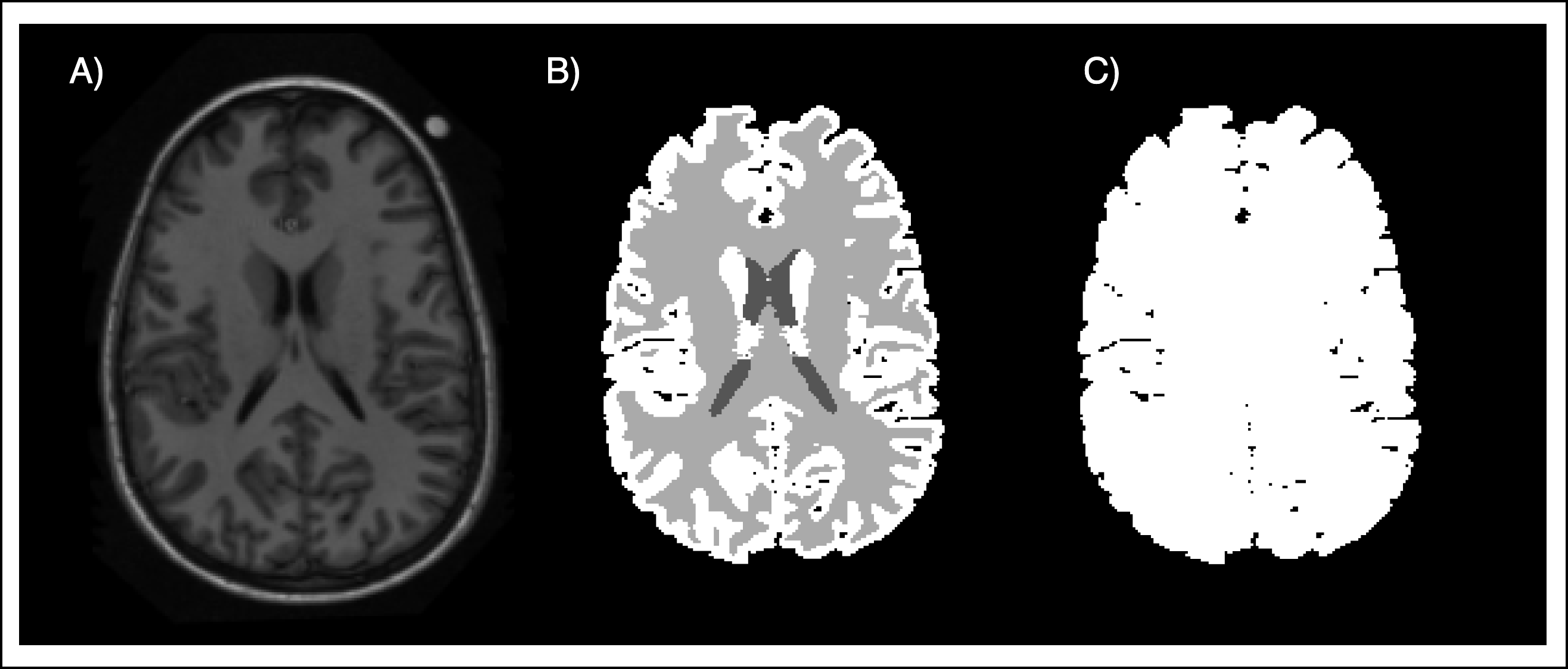
The atlas was built out of 15 different T1 scans of the brain. In addition to the T1 scans, segmentation masks for background, cerebrospinal fluid (CSF), white matter (WM), and grey matter (GM) were provided.
Building the Atlas
In order to build the atlas, all images need to be registered to the same image. But what image should I choose as the fixed image? In general, the image most similar to all others will allow for easier registration and better performance. To locate the fixed image, comparisons between images can be conducted using similarity metrics like mean square error or mutual information.
Registration
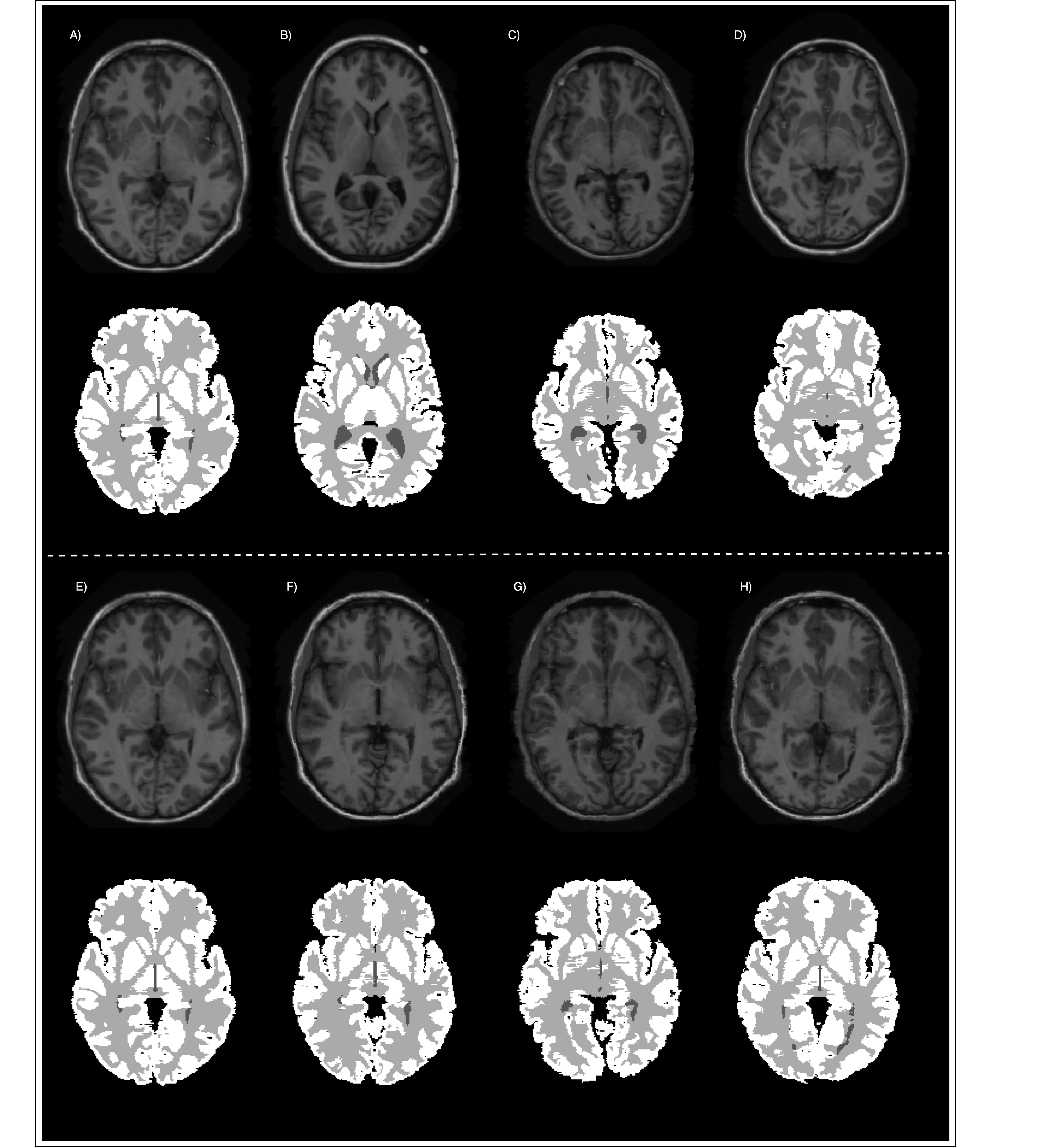
The registrations were carried out using itk-elastix. First, the images are registered rigidly. Secondly, the images are registered with an affine registration. Thirdly, a b-spline multi- resolution registration is performed. Here, an image pyramid with six levels is chosen. Each level’s resolution is half of the previous level. Furthermore, an advanced normalised correlation metric with a transform bending energy penalty is chosen. The parameters as well as the authors can be found on ModelZoo.
Label Propagation
The next step is label propagation. In the previous step, we computed the transformation parameters for the intensity parameters. Now we need to apply this transformation to the masks. In order to avoid the mixing of different tissues, i.e., interpolation errors, the transformations are computed separately.
Putting everything together
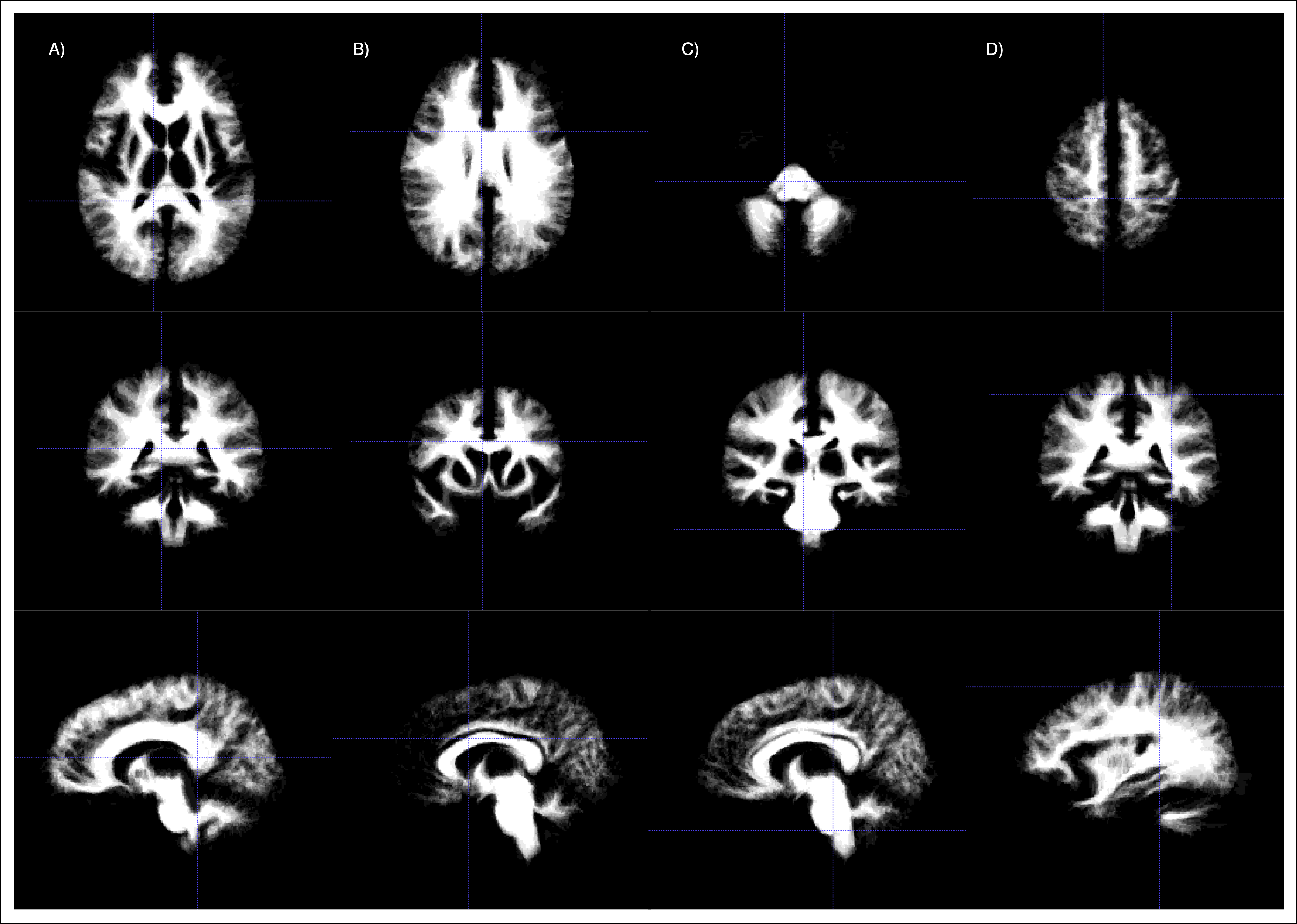
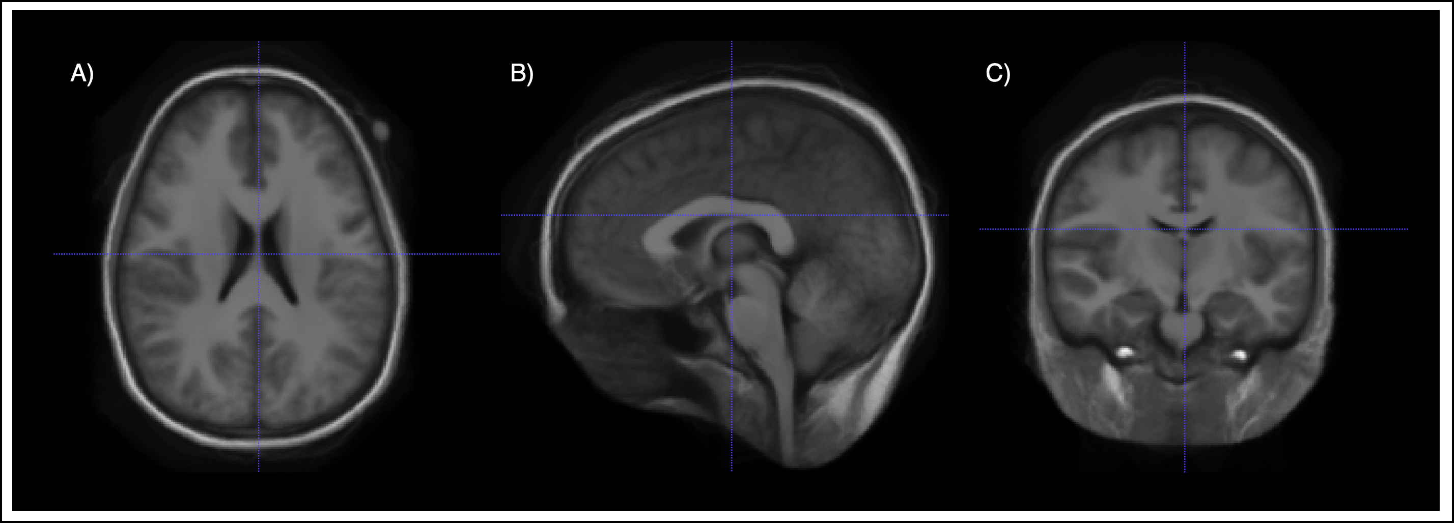
Having applied the transormation to the mask, the atlas can be computed. For this, the voxel-wise mean for each propagated tissue mask is taken. This mean can be interpreted as a probability of a voxel belonging to the tissue. Further, we need to provide an image to allow for registration with the atlas. For this, the mean of all intensity images is taken.
Building the tissue model
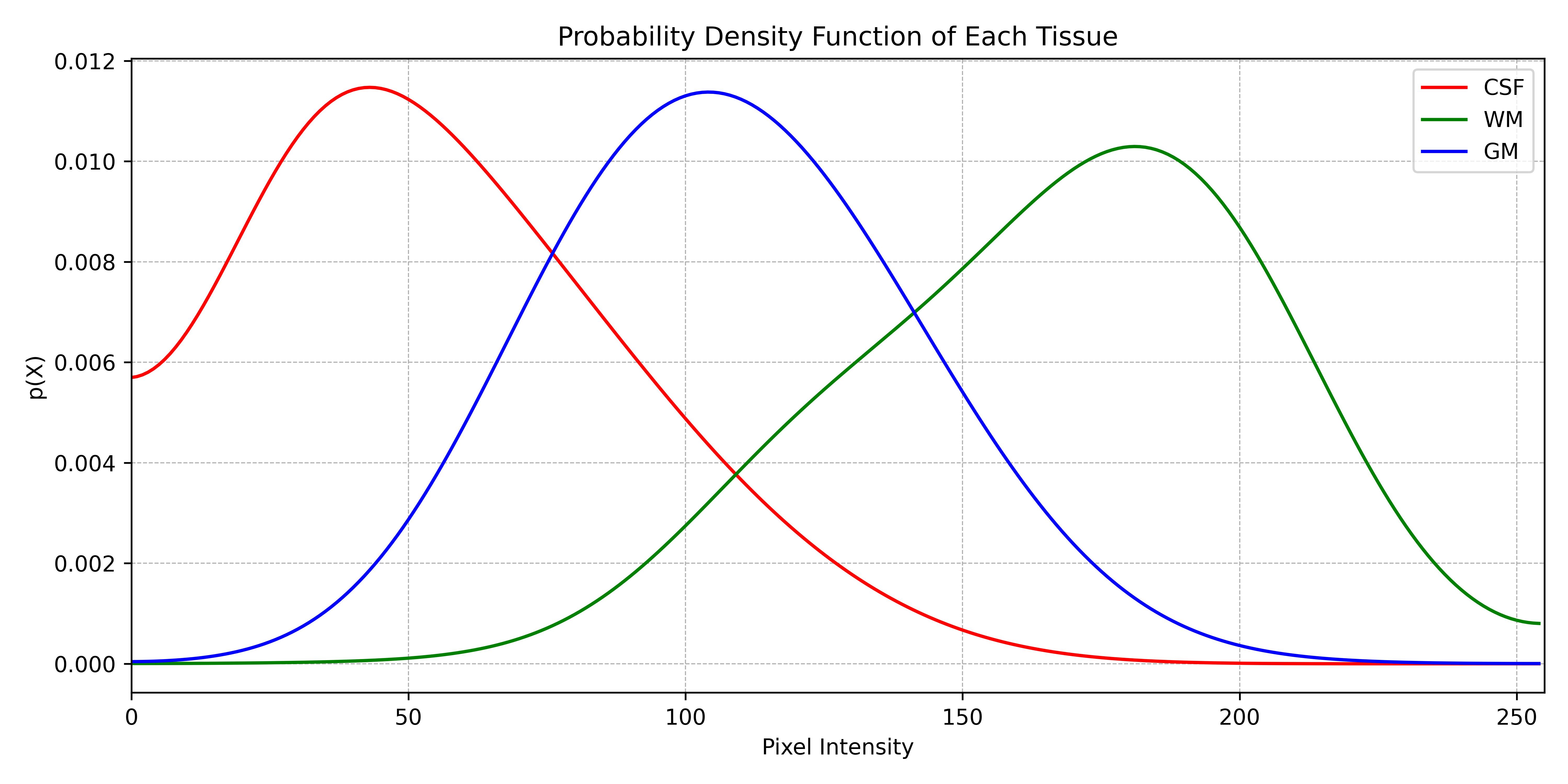
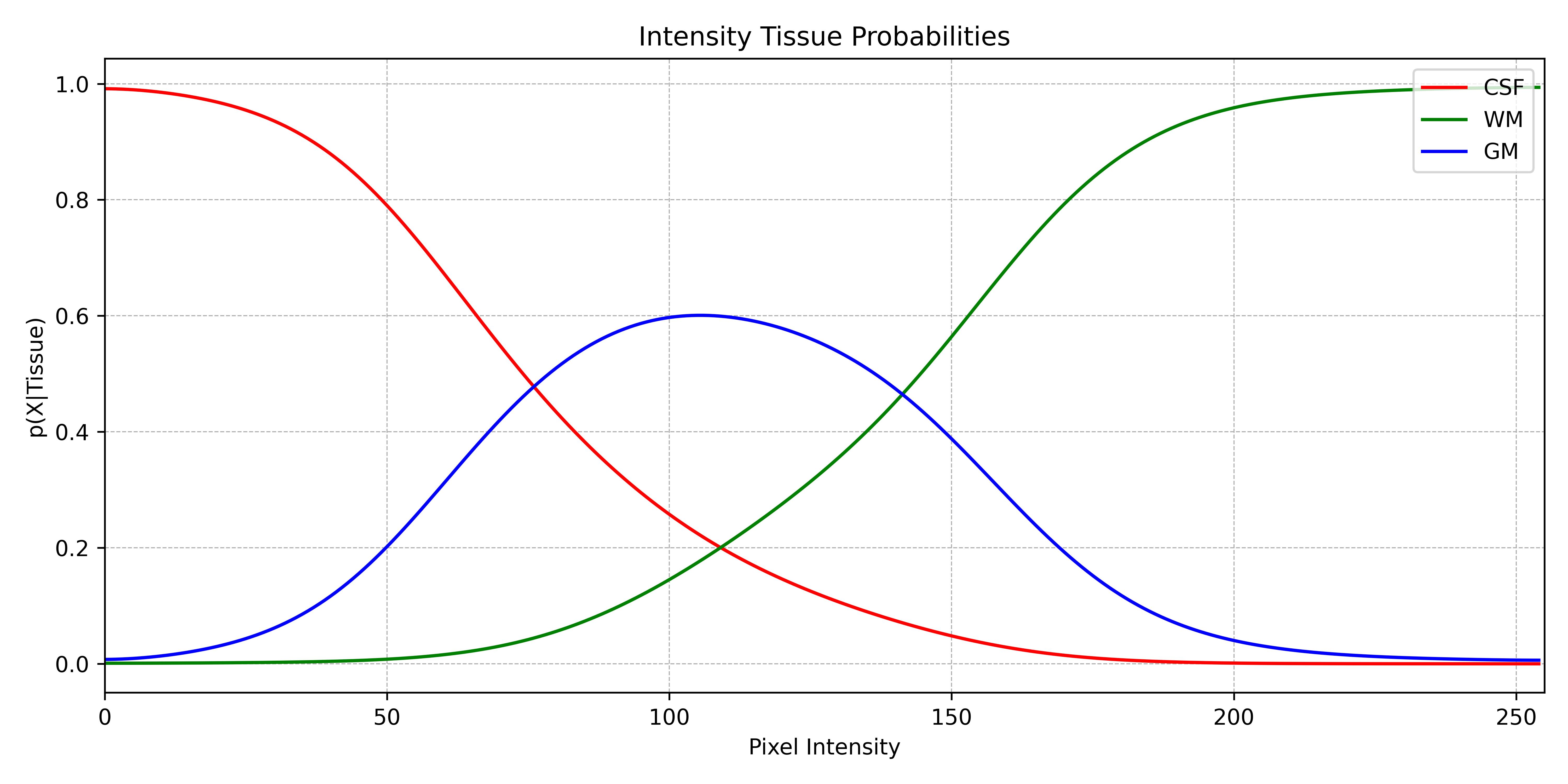
While the atlas provided a probability based on the spatial position of a voxel, the tissue model provides a probability based on the intensity of a voxel. In order to accomplish this, the histogram is computed, normalised to a probability density function, and finally converted to a conditional probability, i.e., the probability of a voxel with an intensity x of belonging to a specific tissue. This is called a tissue model.

Conclusion
This research developed an advanced method for creating a detailed probabilistic brain atlas and tissue probability models using image registration techniques. Our approach, from rigid registration to label propagation, resulted in an atlas with precise tissue boundaries. This work aids in MRI tissue mapping, potentially improving diagnostics. We plan to extend this to more accurate brain tissue segmentation, which could significantly help in neurological diagnosis and treatment.