Lung segmentation in 3D computed tomography scans

Authors: Frederik Hartmann, Yusuf Baran Tanrıverdi
Code: Github

This project was carried out within the scope of the Advanced Image Analysis course taught by Prof. Alessandro Bria. The project was awarded with the best project award 2023. You can reach the more carefully worded report here. Scroll down for a beginner-friendly guide.

April 2023

A detailed tutorial

In this tutorial, it is explained how to segment a lung in a 3D CT scan. First, let’s take a look at a CT scan.

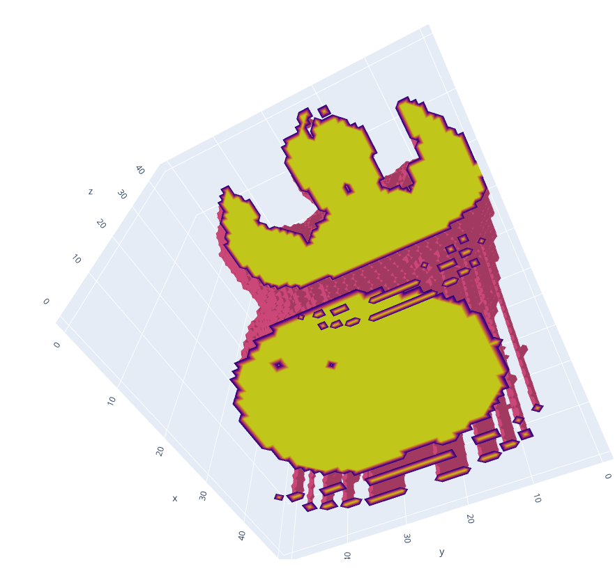
In the picture above, you can vaguely outline the body, head, and arms of the person. Below the person, a table on which the person is lying can be spotted. It is worth mentioning that the table is not broken, and the gaps are due to the display technique used. Now let’s take a look at an axial slice in the centre.

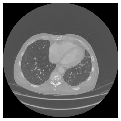
In this image, the lung is displayed in the dark. The surrounding tissues and bones appear brighter. The background has roughly the same intensity as the lung tissue. At the bottom of the picture, multiple lines can be seen. These lines are the edges of the patient table and what appears to be a cushion. The goal of lung segmentation is to find or segment the lung. In order to accomplish this, the table, background, and surrounding tissues need to be removed. In the following, all steps will be explained in detail with text, pictures, and code.

Preprocessing

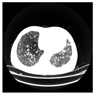
The first step is preprocessing. The goal is to remove the table and make the background have the same intensity as the tissue surrounding the lung. Each pixel or cell in a computed tomography scan is not encoded in a range from 0-255 (8-bit unsigned), but rather in a range from −32,768 to 32,767 (16-bit signed). However, there is more to it. Each value represents a Hounsfield unit (HU), and Hounsfield units can be attributed to a specific tissue. Because we are only interested in lung tissue, we choose a range in which the lung is safely included and set all other pixels to the maximum of the range. In this case, a range of -1000 HU to -500 HU.

def clipScanToHounsfieldUnitRange(scan,HounsfieldUnitRange):
	HU_min = HounsfieldUnitRange[0]
	HU_max = HounsfieldUnitRange[1]
	return np.clip(scan,a_min=HU_min, a_max=HU_max)

This is done for the entire scan. The steps after this are applied to each slice separately. It can be seen that the table in this viewing direction is not a straight line. This will become important later. To make the table straight, we use the sagittal view and therefore use sagittal slices. First we loop through the sagittal slices:

def createMaskForEachSliceOf(self, clippedScan):
	mask = np.zeros(clippedScan.shape, dtype="int16")
	numberOfSagittalSlices = clippedScan.shape[1]
		for i in range(0,numberOfSagittalSlices):
			sagittalSlice = clippedScan[:,:,i]
			sliceMask = self.createMaskFrom(sagittalSlice)
			mask[:,:,i] = sliceMask.astype("int16")
	return mask

The next step is to create a mask for each sagittal slice. Each function will be explained in the following steps.

def createMaskFrom(self,SagittalSlice):
        denoisedSagittalSlice = cv2.medianBlur(SagittalSlice,ksize=5)
        binarizedSagittalSlice = self.binarize(denoisedSagittalSlice)
        sliceWithOpenTable = self.openTableOf(binarizedSagittalSlice)
        SagittalSliceWithUniformBackground, backgroundMask = self.createUniformBackgroundOf(binarizedSagittalSlice)
        mask = self.createMaskByFillingHolesOf(SagittalSliceWithUniformBackground)
        combinedMask = self.combineMasks(mask, backgroundMask)
        return combinedMask

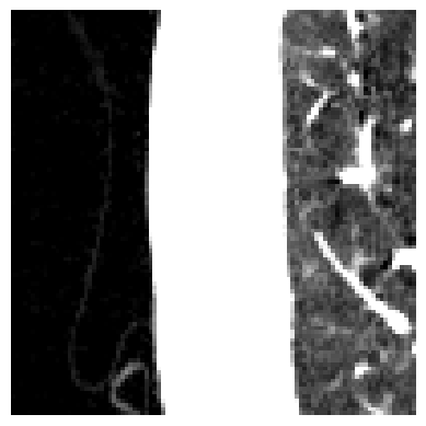
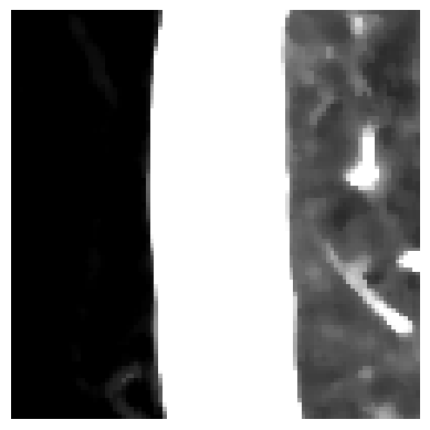
Let’s start with the denoising. It is worth noting that denoising might remove relevant medical information. However, some scans can be a bit noisy. The type of noise seems to be “salt” and “pepper” noise. To reduce this kind of noise, one can apply median filtering. Let’s zoom in on our slice and apply denoising. To the left, you can see the background with some clothes; in the middle, the tissues surrounding the lung; and on the right, the lung. You can see that the noise has been reduced, but at the same time, the slice appears to be more blurry.

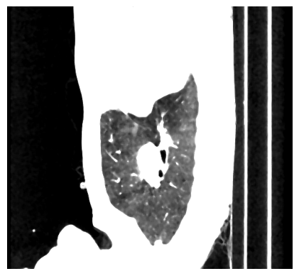
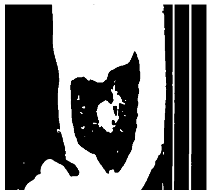
In order to create the mask, we have to binarize the image. The binarization is achieved by thresholding the image with a threshold of the maximum value minus one.

def binarize(sagittalSlice):
	_, binarizedSlice = cv2.threshold(sagittalSlice,
	    	thresh=sagittalSlice.max()-1, maxval=1,
	    	type=cv2.THRESH_BINARY)
	return binarizedSlice.astype("uint8")

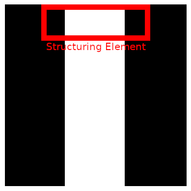
The next goal is to make everything that is not lung tissue white. In order to accomplish this, we will flood the image from the left and right. We could also flood it from the top and bottom, but in case the lung is touching the border, it will flood it to zero. However, a problem remains. When flooding from the right, it is impossible to flow through the table. So we need to break the table first. We do that on the top row of the image only. We use morphological openings to open the table. The structuring element is a line. The line needs to be longer than the table width. The result is displayed below.

def openTableOf(binarizedSagittalSlice):
  kernel = cv2.getStructuringElement(shape=cv2.MORPH_RECT, ksize=(25,1))
  topRowOpen = cv2.morphologyEx(binarizedSagittalSlice[:1], cv2.MORPH_OPEN, kernel, iterations=1)
  binarizedSagittalSlice[:1] = topRowOpen
  return binarizedSagittalSlice)

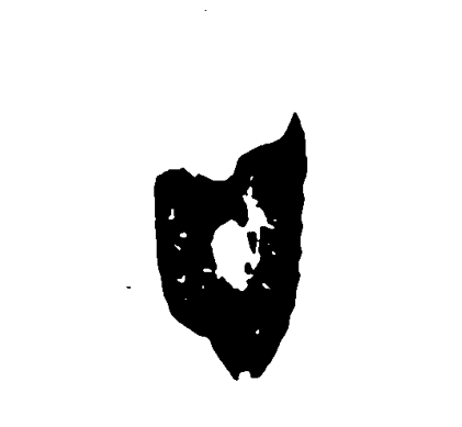
Now we floodfill the binarized image from left to right. In addition to that, we will receive a map of where the floodfilling was applied. We call this mask a background mask. Floodfilling only accepts a single pixel as an input. Since we want to flood from the entire edge, we draw a line in the colour of the background there.

def createUniformBackgroundOf(binarizedSagittalSlice):
  h, w = binarizedSagittalSlice.shape[:2]
  backgroundMask = np.zeros((h+2,w+2),dtype="uint8")
  cv2.line(binarizedSagittalSlice, (0,0),(0,h-1),0,thickness=1) 
  cv2.line(binarizedSagittalSlice, (w-1,0),(w-1,h-1),0,thickness=1) 
  cv2.floodFill(binarizedSagittalSlice, backgroundMask, (0,0),1,flags=4) 
  cv2.floodFill(binarizedSagittalSlice, backgroundMask, (w-1,0),1,flags=4)
  backgroundMask = np.logical_not(backgroundMask[1:-1,1:-1]).astype("uint8") 
  return binarizedSagittalSlice, backgroundMask

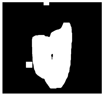
As you can see, we now have the lung in black on a white background. The goal is to have the lung in white on a black background. Because we will apply the mask to the original image again and refine it, we can now close the holes generously. This is done by applying a box filter of ones with a kernel size of 30. The output of this convolution will not be binary anymore. Therefore, the slice is thresholded again. As you can see, the lung area is covered, but there are some points that clearly aren’t below the lung.

def createMaskByFillingHolesOf(BinarySliceWithUniformBackground):
  inverted = (np.logical_not(BinarySliceWithUniformBackground)).astype("uint8")
  filled = cv2.boxFilter(inverted, ddepth=-1, ksize=(30,30), normalize=False)
  _, binarized = cv2.threshold(filled, thresh=1, maxval=1, type=cv2.THRESH_BINARY)
  return binarized

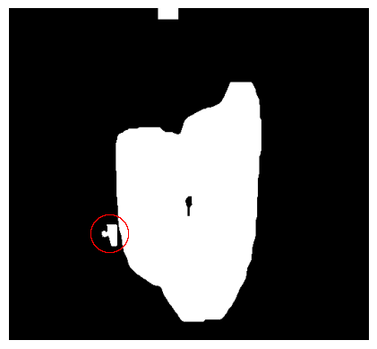
The final step of the preprocessing is the combining of the masks. The creation of the mask in step 7 has caused the mask to grow back in the background. Luckily for us, in step 6, we have created a background mask, so we can just use this one. In the image below, one difference is circled.

def combineMasks(filledMask, backgroundMask):
  return cv2.bitwise_and(filledMask, backgroundMask)

Now let’s put everything together. First, we clip the scan, then we create a mask slice-by-slice by applying the eight steps:

def createCoarseLungMaskOf(self,scan):
  HounsfieldUnitRange = (-1000, -500)
  clippedScan = self.clipScanToHounsfieldUnitRange(scan, HounsfieldUnitRange)
  mask = self.createMaskForEachSliceOf(clippedScan)
  return mask

As a reminder, the returned mask is a 3D numpy array. Additionally, all functions have been put into a class.

Evaluation of preprocessing

The goals of the preprocessing were:

1. Remove the table
2. Make the backgroud and surrounding tissue of the lung the same colour.

Let’s check if the table has been removed:

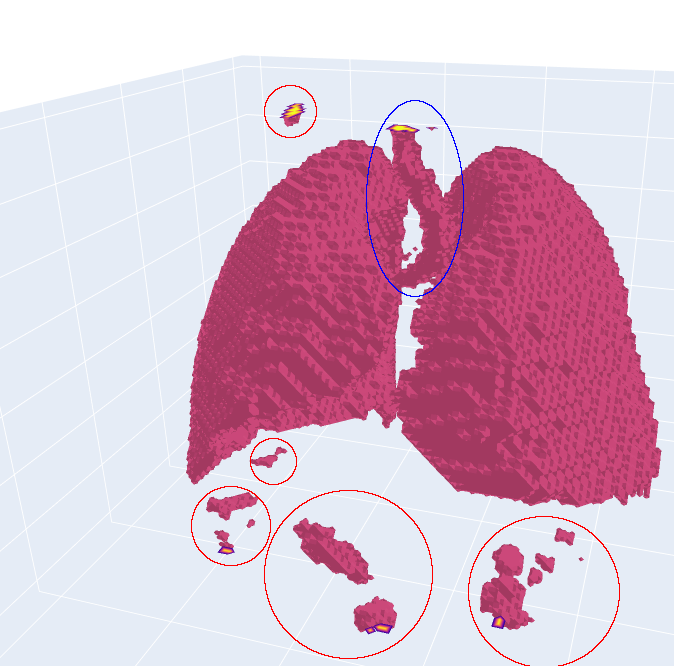
It can be seen that the table was successfully removed. However, some artefacts remain (circled in red). Additionally, the tube in the middle (circled in blue) is not a part of the lung, but it is part of the airways that provide the lung with air. The tube is called the trachea. We will take care of these problems in the next step, but for now, let’s have a look at the background. It can be seen that the background seems to be the same colour, but did we remove any lung ixels or voxels? For that, we calculate the sensitivity on the vessel12 dataset:

It can be seen that some pixels are wrongly labeled as not lung. Nevertheless, the amount of wrongly labeled pixels is low. Additionally, the region of interest has been reduced from the entire image to a smaller mask. The average relative size is

This means that the predicted mask is roughly 81% smaller than the original image.

Lung Segmentation

In the preprocessing step, we have managed to get a relatively coarse lung mask. Let’s refine this mask. The two main goals are:

1. Remove the artefacts.
2. Remove the tracha and aerial ways.

Loading the scan

Before we get into that, There is one thing we haven’t talked about yet, and that is loading the scan. This step now depends on the data format you are using. If you are using Vessel12, the file ending is “mhd”. We can load this file format using SimpleITK. It is worth noting that simpleITK supports a variety of file formats, so just try yours. The “.mhd” file contains meta data and the scan:

 
def readScanMetaFrom(scanPath):
  return sitk.ReadImage(scanPath)

To get the actual scan without meta data, we can use the following:

def readScanMetaFrom(scanPath):
  return sitk.ReadImage(scanPath)

Now we are good to go. So let’s dive right into it. First, we use preprocessing and apply mask the scan:

 
coarseMask = self.preprocessing.createCoarseLungMaskOf(self.scan)
coarseScan = coarseMask*self.scan

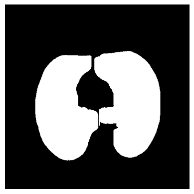
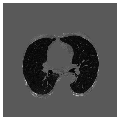
Remember, we want to refine the mask, right? So let’s create a function for that. The idea is the following: We clip the slice again, search for contours, and decide if these contours are lung or not. We will do this by tracking the contours, but more on that later. The process of deciding if a contour is a lung or not is included in the createFineMaskFrom(…) function.

def refine(self, coarseScan):
  HounsfieldUnitRange = (-1000, -500)
  clippedScan = self.preprocessing.clipScanToHounsfieldUnitRange(coarseScan, HounsfieldUnitRange)
  contoursForEachAxialSlice = self.findContoursForEachAxialSliceOf(clippedScan)
  fineMask = self.createFineMaskFrom(contoursForEachAxialSlice)
  return fineMask

Finding Contours

We have covered the clipping in the preprocessing, so the next step is finding the contours. We will search for the contours in the axial slices.

Loop through the axial slices:

def findContoursForEachAxialSliceOf(self, clippedScan):
  numberOfAxialSlices = clippedScan.shape[0]
  contoursForEachAxialSlice = [None] * numberOfAxialSlices
  for i in range(0, numberOfAxialSlices):
      axialSlice = clippedScan[i]
      sliceContours = self.findContoursOf(axialSlice)
      contoursForEachAxialSlice[i] = sliceContours
  return contoursForEachAxialSlice

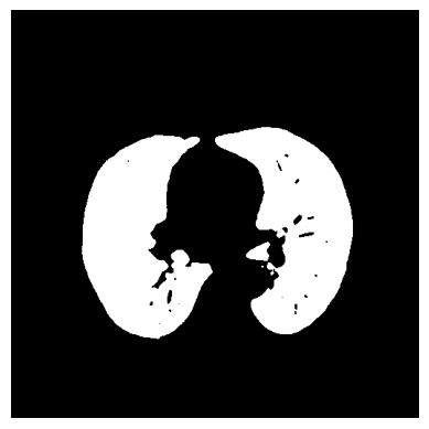
The second step is to find the contours for each axial slice. We will use OpenCV’s findContours for this. Let’s take a look at what the documentation is saying about the input image: Source: an 8-bit single-channel image. Non-zero pixels are treated as 1’s. Zero pixels remain 0’s, so the image is treated as “binary. This is important. The input image will be “converted” to binary. Why not make it binary in the way we want it? Another important thing is not explicitly stated: The background is expected to be black and the foreground to be white. Our background is white, and the foreground—the lung—is black. This will cause findContours to find a contour around the entire image. We don’t want that. Summing up, we have three things to consider:

• The slice should be binary.
• The background should be black and the foreground white.
• The slice should be 8-bit. We will deal with the first two together. First, we denoise the image, and then we threshold the image. This time we use THRESH_BINARY_INV to invert the colors. The lung is now white, and the background is black. After that, we convert the binary image to 8-bit. Let’s take a look at the code and the output image.

def prepare(self, axialSlice):
	denoisedAxialSlice = cv2.medianBlur(axialSlice, ksize=5)
	binarizedAxialSlice = self.binarize(denoisedAxialSlice)
	return binarizedAxialSlice

@staticmethod
def binarize(axialSlice):
	_, binarizedSlice = cv2.threshold(axialSlice, thresh=axialSlice.max()-1,
					maxval=1, type=cv2.THRESH_BINARY_INV)
  	return binarizedSlice.astype("uint8")

Now that we have prepared our slice, it is time to find the contours. But how many lung contours can realistically be in an axial slice? You might think two lungs are two contours. However, this is only the case in three dimensions. The maximum number of lung contours is empirically chosen to be four. We will first look at the code and then at two examples of the contours. Additionally, we use RETR_EXTERNAL to retrieve only the outer contours.

def findContoursOf(self, axialSlice):
  preparedSlice = self.prepare(axialSlice)
  contours,_ = cv2.findContours(preparedSlice, mode=cv2.RETR_EXTERNAL, method=cv2.CHAIN_APPROX_NONE)
  contoursSortedByLength = sorted(contours, key=lambda contour:len(contour), reverse=True)
  reducedNumberOfContours = self.reduceNumberOf(contoursSortedByLength)
  return reducedNumberOfContours

def reduceNumberOf(self, contoursSortedByLength):
  if len(contoursSortedByLength) > self.MAX_NUMBER_OF_CONTOURS_TO_BE_TRACKED:
      return contoursSortedByLength[:self.MAX_NUMBER_OF_CONTOURS_TO_BE_TRACKED]
  else:
      return contoursSortedByLength

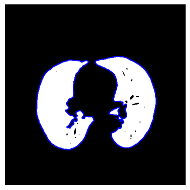
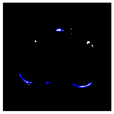
We will take a look at how many contours are correct in the right example later on.

Tracking the Contours

We now have a bunch of contours, but which ones are actually lung contours? Which ones are artifacts? Which ones are tracheas? For this, we will track the contours. We start in the centre slice and assume all contours there are lung contours. We now go one slice up and compare the contours to see if they are more or less the same—it is a lung contour too! We now go on to slice up again and compare the contours to the ones in the slice below, and so on. We will do exactly the same from the centre to the bottom; it is just reversed. Let’s get into it.

First, we create one model for the top half of the 3D image and one for the bottom half.

def createFineMaskFrom(self, contoursForEachAxialSlice):
  refinedBottomMask = self.refineMaskBytrackingLungContours(contoursForEachAxialSlice, direction="centerToTop")
  refinedTopMask = self.refineMaskBytrackingLungContours(contoursForEachAxialSlice, direction="centerToBottom")
  refinedMask = self.addMasks(refinedBottomMask,refinedTopMask)
  return refinedMask

Now we cycle through each axial slice contour by contour and compare it to the counters of the previous slice. Don’t worry too much about the code at the top. The important steps are happening in the for loop. For a closer look at the top functions,refer to this file.

def refineMaskBytrackingLungContours(self, contoursForEachAxialSlice, direction):
  startIndex = self.getStartIndex(contoursForEachAxialSlice, direction)
  finalIndex = self.getFinalIndex(contoursForEachAxialSlice, direction)
  stepDirection = self.stepDirectionToInteger(direction)
  refinedMask = np.zeros(self.scanDimensions)
  centerContours = contoursForEachAxialSlice[startIndex]
  previousMasks = self.getCandidateMasksFrom(centerContours)
  for i in range(startIndex, finalIndex, stepDirection):
	CurrentContours = contoursForEachAxialSlice[i]
	lungMasks = self.comparePreviousMasksToCurrentContours(previousMasks,CurrentContours)
	lungMask = self.createSingleMaskFrom(lungMasks)
	refinedMask[i] = lungMask
	previousMasks = lungMasks
  return refinedMask

For the comparison, we will need a mask rather than a contour. getCandidateMasksFrom is doing just that. We will have a look at it next, also with pictures. After that, we compare every current mask to the masks from the previous slice. Once we have found a match, we assume it is a lung mask. We will not quit the search for this current mask and continue with the next one. If no match is found, we assume it is not a lung. We will also have a close look at isLungMask and how we decide if it’s a lung mask or not, but first we look at getCandidateMasksFrom.

def comparePreviousMasksToCurrentContours(self, previousMasks,CurrentContours):
  candidateMasks = self.getCandidateMasksFrom(CurrentContours)
  lungMasks = [
  for mask in candidateMasks:
    for prevMask in previousMasks:
      if self.isLungMask(mask, prevMask):
        lungMasks.append(mask)
        break # breaks inner loop
  
  return lungMasks

Let us quickly have a look at the code before we look at some pictures. The idea is simple: We create one mask for each contour.<p

def getCandidateMasksFrom(self, CurrentContours):
  numberOfContours = len(CurrentContours)
  candidateMasks = [None] * numberOfContours
  sliceDimensions = self.scanDimensions[1:3]
  for i in range(0,numberOfContours):
    candidateMask = np.zeros(sliceDimensions, dtype="uint8")
    cv2.drawContours(candidateMask, [CurrentContours[i]], contourIdx=-1, color=1, thickness=cv2.FILLED)
    candidateMasks[i] = candidateMask
  return candidateMasks

And finally some pictures:

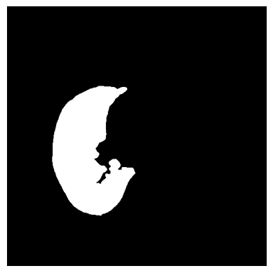
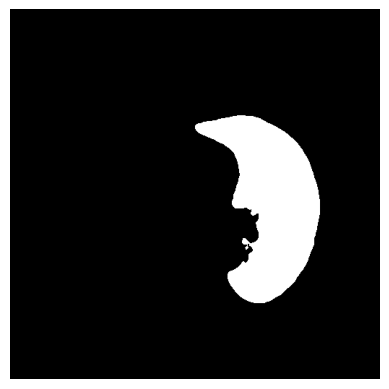
And even more. Remember, we chose the maximum number of contours at four. The tradeoff here is runtime vs. accuracy. The more contours, the higher the runtime, and the higher the accuracy.

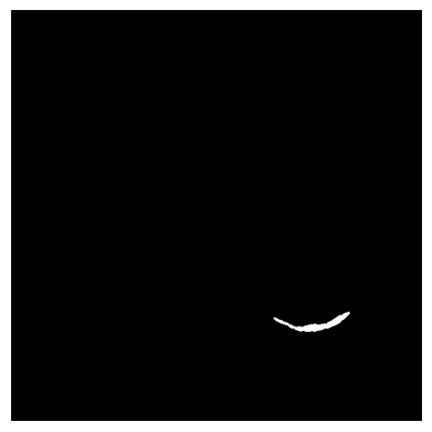
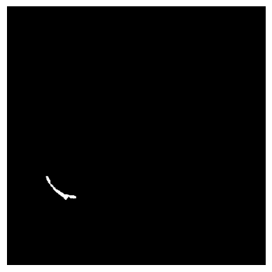
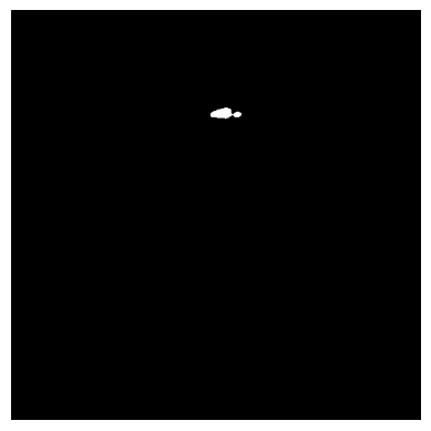
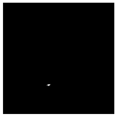
For the comparison, we look at the two Jaccard scores. It accounts for the overlap (intersection) and the union of the current mask and the preceding mask. Instead of the combination, the difference is displayed for visualisation purposes.

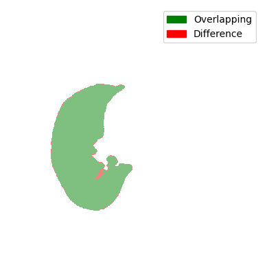
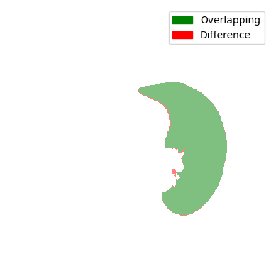
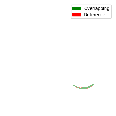
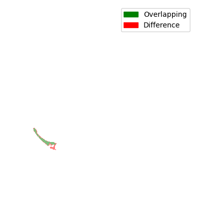
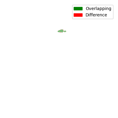
You can see that all comparisons look relatively good. Sure, some differences are a bit bigger and some are a bit smaller, but nonetheless, the difference doesn’t seem that big. So are all of the masks displayed here a lung contour? The answer is shockingly no, because each contour has to be continuously tracked from the centre slice. In the next steps, we will take a look at the decision-making process and the results of the tracking.

For the decision-making process, three cases are considered:

1. Normal case: The contour got slightly bigger or smaller.
2. Splitting Case: One contour split into two contours
3. Merging Case: Two contours merged into one contour Let’s put that into code:

   def isLungMask(self,mask, prevMask):
     jaccardScore = self.computeJaccardScore(mask, prevMask)
     currentSize = cv2.countNonZero(mask)
     prevSize = cv2.countNonZero(prevMask)
     if self.isMaskOverlapping(jaccardScore):
       return True
     elif self.isMaskSplittedIntoTwoMasks(jaccardScorecurrentSize, prevSize):
       return True
     elif self.isMaskMergedFromTwoMasks(jaccardScorecurrentSize, prevSize):
       return True
     else:
       return False
   

Now we need to define each case. But before we do that, let’s look at the Jaccard score:

\begin{equation} jaccard score = intersection / union \end{equation}

We can compute the intersection using an AND Gate, the union using an OR Gate;

def computeJaccardScore(mask, prevMask):
  intersection = cv2.countNonZero(cv2.bitwise_and(mask,prevMask))
  union = cv2.countNonZero(cv2.bitwise_or(mask,prevMask))
  if union != 0:
    return intersection/union
  else:
    return 1.0

Now we can define each case. In the first case, if the Jaccard score is higher than the threshold, which has been set to 0.1, we assume it’s a lung mask.

def isMaskOverlapping(self, jaccardScore):
  if jaccardScore > self.JACCARD_THRESHOLD:
    return True
  else:
    return False

The second case can happen if the two lungs are detected as one contour and then detected as two contours in the next slice. In this case, we assume that the contour is now roughly half as big. The merging is practically the same, but in reverse: two masks merged into one.

def isMaskSplittedIntoTwoMasks(self, jaccardScore, currentSize, prevSize):
  if jaccardScore > self.JACCARD_THRESHOLD/3 and np.isclose(2*currentSize, prevSize, rtol=0.3):
    return True
  else:
    return False

def isMaskMergedFromTwoMasks(self, jaccardScore, currentSize, prevSize):
  if jaccardScore > self.JACCARD_THRESHOLD/3 and np.isclose(currentSize, 2*prevSize, rtol=0.3):
    return True
  else:
    return False

This is an image of an actual splitting case. It is worth noting that the merging case would look the same because we are only displaying the difference and not which slice is the current or previous one. You can see that the lung in the previous slice was one cotour. Now there are two.

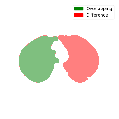
A small Evaluation

Remember the picture with a lot of contours? No? No problem. Here it is again:

Can you guess which ones are lung contours? Let’s take a look at what our tracking predicts:

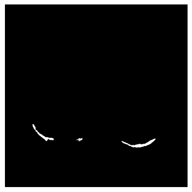
Our tracking presumes the three at the bottom to be lung contours. But is that correct? At the time of writing, I don’t actually know the answer. Let’s compare it to the ground truth to find out.

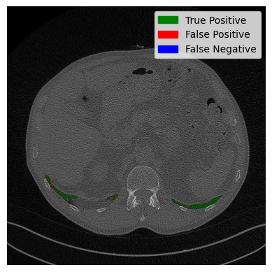
The green part is where our prediction is correct, and the red part has missing pixels. All in all, our tracking was correct, and we identified the three contours correctly. Some pixels are missing, but not too bad. Good stuff.

Postprocessing

The final step is postprocessing. For this, morphological operations in the form of closing are performed.

First we loop through the axial slices

  def closeHolesForEachAxialSlice(self, mask):
    closedMask = np.zeros(mask.shape, dtype="uint8")
    numberOfAxialSlices = mask.shape[0]
    for i in range(0, numberOfAxialSlices):
      closedSlice = self.closeHolesForEachCompoment(mask[i])
      closedMask[i] = closedSlice 
    return closedMask

The closing is performed for each contour/component separately. This will prevent them from growing together.

def closeHolesForEachCompoment(self, axialSlice):
  mask = np.zeros(axialSlice.shape, dtype="uint8")
  numberOfLabels, labelImage = cv2.connectedComponents(axialSlice)
  for label in range(1, numberOfLabels):
    componentImage = np.array(labelImage == label, dtype="uint8")
    closedSlice = self.closeComponent(componentImage)
    mask += closedSlice
  return mask    

And finally the closing:

def closeComponent(componentImage):
  kernel = cv2.getStructuringElement(shape=cv2.MORPH_RECT, ksize=(15,15))  
  return cv2.morphologyEx(componentImage, cv2.MORPH_CLOSE, kernel)

In the figure below, the closing is performed for each component separately and for all components together. You can see that the lung is indirectly connected at the top when no sperate components are used.

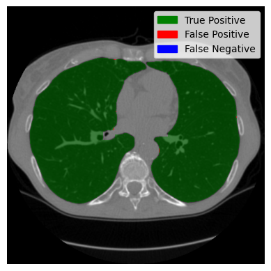
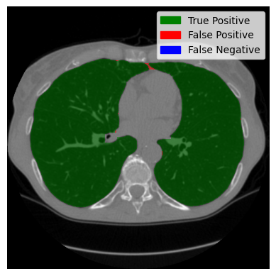
Evaluation

We have now assembled a lung segment. Remember the image we started with? You could still see the person. We reduced our region of interest in the preprocessing and found a lung, but there were artefacts, and the trachea (the tube-looking thing) was still clearly visible. Let’s see if the changes we made were successful:

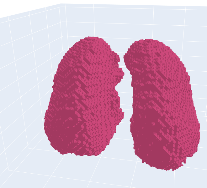
You can see that the artefacts were successfully removed, and the trachea is no longer visible. Let us now take a look at axial slices. We will look at a good-performing example and the worst-performing example I could find.

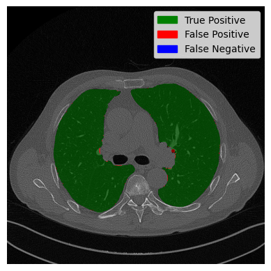
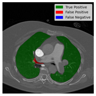
The slice on the left side shows almost perfect segmentation. The overlap between the predicted lung and the actual lung is displayed in green. The two black dots in the middle are the trachea and aerial ways. They were predicted by our algorithm to not be lung. Which is correct? On the right side, the worst case is displayed. A large part of the trachea is wrongly classified as a lung. Now let’s have a look at our image with two contours and see how it did:

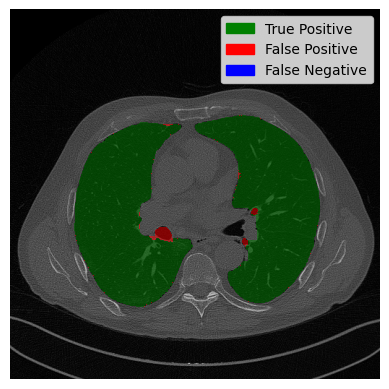
The right lung is mostly classified correctly. Only two small areas of the trachea are wrongly classified. However, on the left side, it can be seen that the trachea was not removed, despite the fact that it is not connected to the lung. The solution to this problem could be retracing the lung from the bottom to the top as the trachea has been correctly removed in the outer parts, which can be seen in the 3D scan or the small evaluation in the preprocessing.

Metrics

Okay, we have seen a lot of slices and scans. Let us put it into numbers now. We will use the Jaccard score as a metric and evaluate it on the Vessel12 dataset. It is worth noting that the Vessel12 dataset is not specifically made for lung segmentation but rather for vessel segmentation. So the results are only to provide an idea of the performance of the algorithm. The dataset consists of twenty CT scans. Let’s see the results:

That doesn’t look too bad!

Limitations

Now we will recap the assumptions we made that ensured the basic functioning, and then we will discuss the problems with the algorithm. In total, three assumptions were made:

• The width in pixels of the table is lower than 25 pixels.
• The lung is surrounded by other tissues from the left and right in sagittal slices.
• All contours in the centre slice are lung.

If the first two conditions are not met, the algorithm will output “randomly”. If the third condition is not met, it will perform worse. A possible lifting of the first condition is the introduction of a width relative to the size of the scan. The third contition could potentially be removed by retracking the lung, as explained above.

The current algorithm has two problems:

1. The thachea in the centre slices is not perfectly removed in some scenarios.
2. The contours do not precisely follow the lung contours if, for example, a vessel is at the edge of the lung.

The origin of the first problem is the third assumption. Hence, it has the same possible solution. The second problem arises from the use of contours to create the mask rather than from the image “directly”. Kmeans has been employed to resample the image. Another less computationally heavy approach is simply the preparation step of the preprocessing—clipping and thresholding. In absence of a perfect ground truth, these approaches have been implemented but could not be evaluated. Therefore, you will not find them in this repository.

Conclusion

All in all, an algorithm for lung segmentation has been successfully implemented. Nevertheless, there is still room for improvement, as described above. I hope you can take something away from this tutorial. Have a great day!